[논문정리] Grad-CAM: Visual Explanations from Deep Networks via Gradient-based Localization

2020. 2. 21. 10:53ㆍPapers/Visualization

Grad-CAM: Visual Explanations from Deep Networks via Gradient-based Localization

Ramprasaath R. Selvaraju, Michael Cogswell, Abhishek Das, Ramakrishna Vedantam, Devi Parikh, Dhruv Batra

Computer Vision and Pattern Recognition (cs.CV); Artificial Intelligence (cs.AI); Machine Learning (cs.LG)

Grad-CAM은 CAM(Class Activation Map)의 확장으로써 기존의 CAM의 경우에는 GAP가 없는 모델의 경우에는 활용할 수 없었지만 Grad-CAM은 gradient (backpropagation과정에서의 기울기를 활용)을 사용함으로써 해당 문제를 해결하였다.

간단하게 Grad-CAM은 어느 Model에서도 활용할 수 있는 장점이 존재한다.

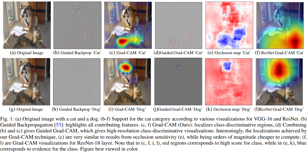
위의 그림을 보면 알 수 있듯이 어떤 class에 대한 Grad-CAM을 보여주냐에 따라서 다른 heat-map이 그려진다. 해당 사진에서는 개와 고양이가 존재하는데 어떤 class에 heat-map을 그리게 할 것인가에 따라서 (c),(i)와 같이 차이가 날 수 있다.

빨간색일수록 강한 영향을 미치는 것을 표현하며, 파란색일수록 적은 영향력을 미치는 것을 나타낸다.

- 해당 이미지에 없는 class에 대해서 Grad-CAM을 그릴 수도 있다. 이는 해당 클래스라고 판단한다면 무엇을 보고 판단하는지에 대한 정보를 시각화하여 보여주는 것을 의미한다.

위의 그림을 보면 알 수 있듯이 Grad-CAM을 만들기 위해서는 Convolutional layer에서의 gradient를 활용하여 해당 gradient와 Convolutional layer's feature maps과 곱연산하여 추가적으로 ReLU Activation function을 거친 값을 input이미지에 heat-map표현을 해주는 것으로 Grad-CAM을 표현할 수 있다.

Guided Backpropagation은 기존의 ReLU Activation function의 backward부분을 Guided부분으로 수정하면 된다.

- 기존의 ReLU는 Forward에서의 값이 0보다 큰 경우 $\frac{{\partial}y}{{\partial}x}=1$이지만 Guided의 경우에는 입력 backward의 input값이 0보다 작은 경우에도 0으로 만들어주는 역할이 존재한다. 해당 부분을 식으로 표현하면 다음과 같다.

$$ReLU's Backpropagation : R_i^l = (f_i^l>0){\cdot}R_i^{l+1}, where R_i^{i+1} = \frac{{\partial}f^{out}}{{\partial}f_i^{l+1}}$$

$$ReLU's Guided Backpropagation : R_i^l = (f_i^l>0)\cdot(R_i^{l+1}>0){\cdot}R_i^{l+1}$$

두 식의 차이점이라면 이전 backpropagation의 값을 활용하냐(0보다 큰지 확인을하냐)의 차이가 존재한다. 이 차이를 통해 시각화를해보면 Guided backpropagation이 기존 backpropagation보다 자연스러운 이미지를 보여줌을 알 수 있다.

Grad-CAM 수식

$$\alpha_k^c=\overbrace{\frac{1}{Z}\sum_i\sum_j}^{global average pooling}\underbrace{\frac{{\partial}y^c}{{\partial}A_{ij}^k}}_{gradients via backprop}$$

$$L^c_{Grad-CAM}=ReLU\underbrace{(\sum_k\alpha_k^cA^k)}_{linear combintation}$$

$$y^c=\sum_k\underbrace{w_k^c}_{class feature weights}\overbrace{\frac{1}{Z}\sum_i\sum_j}^{global average pooling}\underbrace{A^k_{ij}}_{feature map}$$

$$y^c=\frac{1}{Z}{\sum_i}{\sum_j}\underbrace{{\sum_k}{w_k^c}{A_{ij}^k}}_{L_{CAM}^c}$$

$$F_k=\frac{1}{Z}\sum_i\sum_jA_{ij}^k$$

$$y^c=\sum_kw_k^cF_k$$

$$\frac{{\partial}y^c}{{\partial}F_k}=\frac{\frac{{\partial}y^c}{{\partial}A_{ij}^k}}{\frac{{\partial}F_k}{{\partial}A_{ij}^k}}$$

$$\frac{{\partial}F_k}{{\partial}A_{ij}^k}=\frac{1}{Z}$$

$$\frac{{\partial}y^c}{{\partial}F_k}=w_k^c$$

$$\frac{{\partial}y^c}{{\partial}F_k}=w_k^c=Z{\cdot}\frac{{\partial}y^c}{{\partial}A_{ij}^k}$$

$$\sum_i\sum_jw_k^c=Z{\cdot}\sum_i\sum_j\frac{{\partial}y^c}{{\partial}A_{ij}^k}$$

$$Z{\cdot}w_k^c=Z{\cdot}\sum_i\sum_j\frac{{\partial}y^c}{{\partial}A_{ij}^k}$$

$$w_k^c=\sum_i\sum_j\frac{{\partial}y^c}{{\partial}A_{ij}^k}$$

$${\therefore}w_k^c=Z{\cdot}\alpha_k^c$$

위의 식을 통해서 $\alpha_k^c$와 $w_k^c$가 일반화시킨 것을 알 수 있다.

그렇기에 CAM과 Grad-CAM의 결과를 확인하면 일치함을 알 수 있다.

Grad-CAM은 GAP의 제약이 없기 때문에 Feature maps의 channel만 일치한다면 어떤 layer든 시각화를 할 수 있다.

Source

다음부터 나오는 소스는 pytorch로 짜여진 소스임을 알아두시면 좋습니다.

import torch
import cv2
import numpy as np
from torchsummary import summary
from torch.nn import functional as F

class ModelOutputs_resnet():
    def __init__(self, model, target_layers, target_sub_layers):
        self.model = model
        self.target_layers = target_layers
        self.target_sub_layers = target_sub_layers
        self.gradients = []

    def save_gradient(self, grad):
        self.gradients.append(grad)

    def get_gradients(self):
        return self.gradients

    def __call__(self, x):
        self.gradients = []
        for name, module in self.model.named_children(): # 모든 layer에 대해서 직접 접근
            x = module(x)
            if name== 'avgpool': # avgpool이후 fully connect하기 전 data shape을 flatten시킴
                x = torch.flatten(x,1)
            if name in self.target_layers: # target_layer라면 해당 layer에서의 gradient를 저장
                for sub_name, sub_module in module[len(module)-1].named_children():
                    if sub_name in self.target_sub_layers:
                        x.register_hook(self.save_gradient) #
                        target_feature_maps = x # x's shape = 512X14X14(C,W,H) feature map
        return target_feature_maps, x # target_activation : target_activation_layer's feature maps // output : classification ( ImageNet's classes : 1000 )


class GradCam_resnet:
    def __init__(self, model, target_layer_names,target_sub_layer_names, use_cuda):
        self.model = model
        self.model.eval()
        self.cuda = use_cuda
        if self.cuda:  # GPU일 경우 model을 cuda로 설정
            self.model = model.cuda()

        self.extractor = ModelOutputs_resnet(self.model, target_layer_names,target_sub_layer_names)

    def forward(self, input):
        return self.model(input)

    def __call__(self, input, index=None):

        if self.cuda:  # GPU일 경우 input을 cuda로 변환하여 전달
            features, output = self.extractor(input.cuda())
        else:
            features, output = self.extractor(input)

        probs,idx = 0, 0
        if index == None:
            index = np.argmax(output.cpu().data.numpy())  # index = 정답이라고 추측한 class index
            h_x = F.softmax(output,dim=1).data.squeeze()
            probs, idx = h_x.sort(0,True)


        one_hot = np.zeros((1, output.size()[-1]), dtype=np.float32)
        one_hot[0][index] = 1  # 정답이라고 생각하는 class의 index 리스트 위치의 값만 1로
        one_hot = torch.from_numpy(one_hot).requires_grad_(True)  # numpy배열을 tensor로 변환
        # requires_grad == True 텐서의 모든 연산에 대하여 추적
        if self.cuda:
            one_hot = torch.sum(one_hot.cuda() * output)
        else:
            one_hot = torch.sum(one_hot * output)

        self.model.zero_grad()
        one_hot.backward(retain_graph=True)

        grads_val = self.extractor.get_gradients()[-1].cpu().data.numpy()

        target = features  # A^k

        target_cam = target.cpu().data.numpy()
        bz, nc, h,w = target_cam.shape

        target = target.cpu().data.numpy()[0, :]

        params = list(self.model.parameters())

        weight_softmax = np.squeeze(params[-2].data.cpu().numpy())

        cam = weight_softmax[index].dot(target_cam.reshape((nc,h*w)))
        cam = cam.reshape(h,w)
        cam = np.maximum(cam, 0)
        cam = cv2.resize(cam, (224, 224))  # 224X224크기로 변환
        cam = cam - np.min(cam)
        cam = cam / np.max(cam)


        weights = np.mean(grads_val, axis=(2, 3))[0, :]  # 논문에서의 global average pooling 식에 해당하는 부분
        grad_cam = np.zeros(target.shape[1:], dtype=np.float32)  # 14X14

        for i, w in enumerate(weights): # calcul grad_cam
            grad_cam += w * target[i, :, :]  # linear combination L^c_{Grad-CAM}에 해당하는 식에서 ReLU를 제외한 식

        grad_cam = np.maximum(grad_cam, 0)  # 0보다 작은 값을 제거
        grad_cam = cv2.resize(grad_cam, (224, 224))  # 224X224크기로 변환
        grad_cam = grad_cam - np.min(grad_cam)  #
        grad_cam = grad_cam / np.max(grad_cam)  # 위의 것과 해당 줄의 것은 0~1사이의 값으로 정규화하기 위한 정리
        return grad_cam, cam ,index,probs,idx ,

pytorch.models의 resnet모델의 경우에는 block이 sequential로 묶여져 있기 때문에 VGG와는 사뭇 다르게 접근해야 한다. 특히 추후에 나올 Guided Backprop에서 ReLU 역전파를 수정할 때 주의해야 함.

VGG의 경우에는 몇번째 layer로 바로 접근이 가능하지만 ResNet의 경우에는 몇번째 block인지를 판단하고 해당 block에서 마지막 conv의 feature map과 gradient를 가져오는 작업을 한다. layer4에 있는 conv2 접근하여 gradient와 feature map을 가져온다.

import torch
import cv2
import numpy as np



from torch.nn import functional as F


class FeatureExtractor_vgg():
    """ Class for extracting activations and
    registering gradients from targetted intermediate layers """

    def __init__(self, model, target_layers): # target_layers = 35 ==> VGG19에서 가장 마지막 MaxPool2D전 ReLU함수
        self.model = model
        self.target_layers = target_layers
        self.gradients = []

    def save_gradient(self, grad):
        self.gradients.append(grad)


    def __call__(self, x):
        self.gradients = []
        for name, module in self.model._modules.items(): # 모든 layer에 대해서 직접 접근
            x = module(x)
            if name in self.target_layers: # target_layer라면 해당 layer에서의 gradient를 저장
                x.register_hook(self.save_gradient) #
                target_feature_maps = x # x's shape = 512X14X14(C,W,H) feature map
        return target_feature_maps, x


class ModelOutputs_vgg():
    """ Class for making a forward pass, and getting:
    1. The network output.
    2. Activations from intermeddiate targetted layers.
    3. Gradients from intermeddiate targetted layers. """

    def __init__(self, model, target_layers):
        self.model = model
        self.feature_extractor = FeatureExtractor_vgg(self.model.features, target_layers)

    def get_gradients(self):
        return self.feature_extractor.gradients

    def __call__(self, x):
        target_activations, output = self.feature_extractor(x)
        output = output.view(output.size(0), -1)
        output = self.model.classifier(output) # feature extract를 통해서 나온 값을 활용하여 classification 진행
        #print("ModelOutputs().output.shape : ",output[0])
        #print("ModelOutputs().target_activations.shape :",target_activations[0])
        return target_activations, output

class GradCam_vgg:
    def __init__(self, model, target_layer_names, use_cuda):
        self.model = model
        self.model.eval()
        self.cuda = use_cuda
        if self.cuda: # GPU일 경우 model을 cuda로 설정
            self.model = model.cuda()

        self.extractor = ModelOutputs_vgg(self.model, target_layer_names)

    def forward(self, input):
        return self.model(input)

    def __call__(self, input, index=None):
        if self.cuda: # GPU일 경우 input을 cuda로 변환하여 전달
            features, output = self.extractor(input.cuda())
        else:
            features, output = self.extractor(input)
        #print("features : ",features.cpu().data.numpy().shape) # 해당 위치에서 추출된 feature map ( 512,14,14 ) (ChannelX14X14)
        #print("output : ",output.cpu().data.numpy().shape) # class를 의미함
        probs, idx = 0,0
        #print("index : ", index)
        if index == None:
            index = np.argmax(output.cpu().data.numpy())  # index = 정답이라고 추측한 class index
            h_x = F.softmax(output,dim=1).data.squeeze()
            probs, idx = h_x.sort(0,True)
        #print("index : ", index)
        one_hot = np.zeros((1, output.size()[-1]), dtype=np.float32)
        one_hot[0][index] = 1 # 정답이라고 생각하는 class의 index 리스트 위치의 값만 1로
        one_hot = torch.from_numpy(one_hot).requires_grad_(True) # numpy배열을 tensor로 변환
        # requires_grad == True 텐서의 모든 연산에 대하여 추적
        if self.cuda:
            one_hot = torch.sum(one_hot.cuda() * output)
        else:
            one_hot = torch.sum(one_hot * output)

        self.model.features.zero_grad()
        self.model.classifier.zero_grad()
        one_hot.backward(retain_graph=True)

        grads_val = self.extractor.get_gradients()[-1].cpu().data.numpy()
        #print("grads_val : ",grads_val.shape) # 512 X 14 X 14
        target = features  # A^k
        target = target.cpu().data.numpy()[0, :]

        cam = None

        weights = np.mean(grads_val, axis=(2, 3))[0, :]  # 논문에서의 global average pooling 식에 해당하는 부분
        grad_cam = np.zeros(target.shape[1:], dtype=np.float32)  # 14X14

        for i, w in enumerate(weights):  # calcul grad_cam
            grad_cam += w * target[i, :, :]  # linear combination L^c_{Grad-CAM}에 해당하는 식에서 ReLU를 제외한 식

        grad_cam = np.maximum(grad_cam, 0)  # 0보다 작은 값을 제거
        grad_cam = cv2.resize(grad_cam, (224, 224))  # 224X224크기로 변환
        grad_cam = grad_cam - np.min(grad_cam)  #
        grad_cam = grad_cam / np.max(grad_cam)  # 위의 것과 해당 줄의 것은 0~1사이의 값으로 정규화하기 위한 정리
        return grad_cam, cam, index, probs, idx,

VGG같은 경우에는 35번째 layer가 마지막 conv이기 때문에 해당 index에서 gradient와 feature maps을 활용하면 된다.

그 외의 작업은 ResNet과 동일하다.

결과

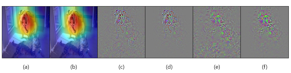
위의 결과를 보면 알 수 있듯이 일반적인 ReLU Backprop일 경우에는 이미지의 전체적인 형태가 뭉개지게 된다. 따라서 Guided Backprop을 활용하면 그림 (c),(d)와 같이 얻을 수 있다. Guided Backprop과 일반 ReLU의 차이점은 backward 과정에서 input의 크기만 신경쓰는 것이 일반적인 ReLU이며 Guided Backprop은 backward의 입력의 값의 크기 또한 양수여야 기존의 값을 유지하는 방법이다.